Create Autoregressive Moving Average Models
These examples show how to create various autoregressive moving average
(ARMA) models by using the arima function.
Default ARMA Model
This example shows how to use the shorthand arima(p,D,q) syntax to specify the default ARMA(p, q) model,
By default, all parameters in the created model object have unknown values, and the innovation distribution is Gaussian with constant variance.
Specify the default ARMA(1,1) model:
Mdl = arima(1,0,1)
Mdl =
  arima with properties:

     Description: "ARIMA(1,0,1) Model (Gaussian Distribution)"
      SeriesName: "Y"
    Distribution: Name = "Gaussian"
               P: 1
               D: 0
               Q: 1
        Constant: NaN
              AR: {NaN} at lag [1]
             SAR: {}
              MA: {NaN} at lag [1]
             SMA: {}
     Seasonality: 0
            Beta: [1×0]
        Variance: NaN
The output shows that the created model object, Mdl, has NaN values for all model parameters: the constant term, the AR and MA coefficients, and the variance. You can modify the created model object using dot notation, or input it (along with data) to estimate.
ARMA Model with No Constant Term
This example shows how to specify an ARMA(p, q) model with constant term equal to zero. Use name-value syntax to specify a model that differs from the default model.
Specify an ARMA(2,1) model with no constant term,
where the innovation distribution is Gaussian with constant variance.
Mdl = arima('ARLags',1:2,'MALags',1,'Constant',0)
Mdl =
  arima with properties:

     Description: "ARIMA(2,0,1) Model (Gaussian Distribution)"
      SeriesName: "Y"
    Distribution: Name = "Gaussian"
               P: 2
               D: 0
               Q: 1
        Constant: 0
              AR: {NaN NaN} at lags [1 2]
             SAR: {}
              MA: {NaN} at lag [1]
             SMA: {}
     Seasonality: 0
            Beta: [1×0]
        Variance: NaN
The ArLags and MaLags name-value pair arguments specify the lags corresponding to nonzero AR and MA coefficients, respectively. The property Constant in the created model object is equal to 0, as specified. The model has default values for all other properties, including NaN values as placeholders for the unknown parameters: the AR and MA coefficients, and scalar variance.
You can modify the created model using dot notation, or input it (along with data) to estimate.
ARMA Model with Known Parameter Values
This example shows how to specify an ARMA(p, q) model with known parameter values. You can use such a fully specified model as an input to simulate or forecast.
Specify the ARMA(1,1) model
where the innovation distribution is Student's t with 8 degrees of freedom, and constant variance 0.15.
tdist = struct('Name','t','DoF',8);
Mdl = arima('Constant',0.3,'AR',0.7,'MA',0.4,...
    'Distribution',tdist,'Variance',0.15)
Mdl =
  arima with properties:

     Description: "ARIMA(1,0,1) Model (t Distribution)"
      SeriesName: "Y"
    Distribution: Name = "t", DoF = 8
               P: 1
               D: 0
               Q: 1
        Constant: 0.3
              AR: {0.7} at lag [1]
             SAR: {}
              MA: {0.4} at lag [1]
             SMA: {}
     Seasonality: 0
            Beta: [1×0]
        Variance: 0.15
All parameter values are specified, that is, no object property is NaN-valued.
Specify ARMA Model Using Econometric Modeler App
In the Econometric Modeler app, you can specify the lag structure, presence of a constant, and innovation distribution of an ARMA(p,q) model by following these steps. All specified coefficients are unknown but estimable parameters.
At the command line, open the Econometric Modeler app.
econometricModeler
Alternatively, open the app from the apps gallery (see Econometric Modeler).
In the Time Series pane, select the response time series to which the model will be fit.
On the Econometric Modeler tab, in the Models section, click ARMA.
The ARMA Model Parameters dialog box appears.
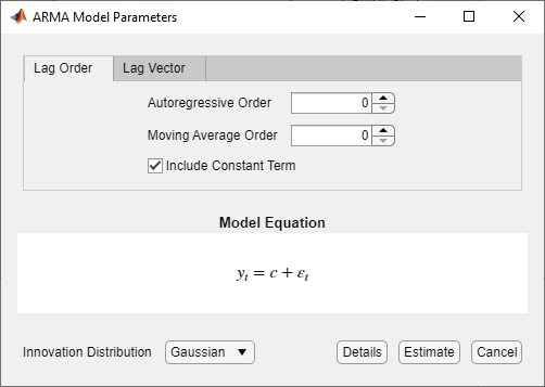
Specify the lag structure. To specify an ARMA(p,q) model that includes all AR lags from 1 through p and all MA lags from 1 through q, use the Lag Order tab. For the flexibility to specify the inclusion of particular lags, use the Lag Vector tab. For more details, see Specifying Univariate Lag Operator Polynomials Interactively. Regardless of the tab you use, you can verify the model form by inspecting the equation in the Model Equation section.
For example:
To specify an ARMA(2,1) model that includes a constant, includes all AR and MA lags from 1 through their respective orders, and has a Gaussian innovation distribution:
Set Autoregressive Order to
2.Set Moving Average Order to
1.
To specify an ARMA(2,1) model that includes all AR and MA lags from 1 through their respective orders, has a Gaussian distribution, but does not include a constant:
Set Autoregressive Order to
2.Set Moving Average Order to
1.Clear the Include Constant Term check box.
To specify an ARMA(2,1) model that includes all AR and MA lags from 1 through their respective orders, includes a constant term, and has t-distributed innovations:
Set Autoregressive Order to
2.Set Moving Average Order to
1.Click the Innovation Distribution button, then select
t.
The degrees of freedom parameter of the t distribution is an unknown but estimable parameter.
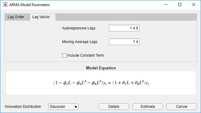
To specify an ARMA(8,4) model containing nonconsecutive lags
where εt is a series of IID Gaussian innovations:
Click the Lag Vector tab.
Set Autoregressive Lags to
1 4 8.Set Moving Average Lags to
1 4.Clear the Include Constant Term check box.
After you specify a model, click Estimate to estimate all unknown parameters in the model.
What Are Autoregressive Moving Average Models?
ARMA(p,q) Model
For some observed time series, a very high-order AR or MA model is needed to model the underlying process well. In this case, a combined autoregressive moving average (ARMA) model can sometimes be a more parsimonious choice.
An ARMA model expresses the conditional mean of yt as a function of both past observations, , and past innovations, The number of past observations that yt depends on, p, is the AR degree. The number of past innovations that yt depends on, q, is the MA degree. In general, these models are denoted by ARMA(p,q).
The form of the ARMA(p,q) model in Econometrics Toolbox™ is
| (1) |
In lag operator polynomial notation, . Define the degree p AR lag operator polynomial . Define the degree q MA lag operator polynomial . You can write the ARMA(p,q) model as
| (2) |
The signs of the coefficients in the AR lag operator polynomial, , are opposite to the right side of Equation 1. When specifying and interpreting AR coefficients in Econometrics Toolbox, use the form in Equation 1.
Stationarity and Invertibility of the ARMA Model
Consider the ARMA(p,q) model in lag operator notation,
From this expression, you can see that
| (3) |
is the unconditional mean of the process, and is a rational, infinite-degree lag operator polynomial, .
Note
The Constant property of an arima model
object corresponds to c, and not the unconditional mean
μ.
By Wold’s decomposition [2], Equation 3 corresponds to a stationary stochastic process provided the coefficients are absolutely summable. This is the case when the AR polynomial, , is stable, meaning all its roots lie outside the unit circle. Additionally, the process is causal provided the MA polynomial is invertible, meaning all its roots lie outside the unit circle.
Econometrics Toolbox enforces stability and invertibility of ARMA processes. When you
specify an ARMA model using arima, you get an error if you enter
coefficients that do not correspond to a stable AR polynomial or invertible MA
polynomial. Similarly, estimate imposes stationarity and
invertibility constraints during estimation.
References
[1] Box, George E. P., Gwilym M. Jenkins, and Gregory C. Reinsel. Time Series Analysis: Forecasting and Control. 3rd ed. Englewood Cliffs, NJ: Prentice Hall, 1994.
[2] Wold, Herman. "A Study in the Analysis of Stationary Time Series." Journal of the Institute of Actuaries 70 (March 1939): 113–115. https://doi.org/10.1017/S0020268100011574.
See Also
Apps
Objects
Functions
Related Topics
- Analyze Time Series Data Using Econometric Modeler
- Specifying Univariate Lag Operator Polynomials Interactively
- Creating Univariate Conditional Mean Models
- Modify Properties of Conditional Mean Model Objects
- Specify Conditional Mean Model Innovation Distribution
- Plot the Impulse Response Function of Conditional Mean Model
You can also select a web site from the following list:
Americas
- América Latina (Español)
- Canada (English)
- United States (English)
Europe
- Belgium (English)
- Denmark (English)
- Deutschland (Deutsch)
- España (Español)
- Finland (English)
- France (Français)
- Ireland (English)
- Italia (Italiano)
- Luxembourg (English)
- Netherlands (English)
- Norway (English)
- Österreich (Deutsch)
- Portugal (English)
- Sweden (English)
- Switzerland
- United Kingdom (English)