Use Parallel Computing to Optimize Big Data Set for Analysis
This example shows how to optimize data preprocessing for analysis using parallel computing.
By optimizing the organization, storage of time series data, you can simplify and accelerate any downstream applications like predictive maintenance, digital twins, signal-based AI, and fleet analytics.
In this example, you transform large raw data into a state ready for future analysis and save it to Parquet files using parallel workers. Parquet files offer efficient access to data because they efficiently store column-oriented heterogeneous data, allowing you to conditionally filter the files by row and only load the data you need. Next, you can use the out-of-memory data to train a simple AI model.
If you have data stored on a cluster, you can use this code for similar data optimization without downloading the data. To see an example that performs analysis on data stored in the cloud, see Process Big Data in the Cloud.
Start a parallel pool of process workers.
pool = parpool("Processes");Starting parallel pool (parpool) using the 'Processes' profile ... 15-Jan-2024 12:03:49: Job Running. Waiting for parallel pool workers to connect ... Connected to parallel pool with 6 workers.
Download Flight Data
This example uses sample aircraft sensor data provided by NASA [1].
If you want to try these data preprocessing techniques yourself, you must download the aircraft sensor data. NASA provides data for approximately 180,000 flights, with one MAT file representing each flight. For more information, see Sample Flight Data.
This code creates a folder in your current folder and downloads data for the first year of aircraft tail number 652, which occupies approximately 1.6 GB of disk space. Downloading the data can take several minutes. To confirm that you want to download the data, select "true" from the drop-down list before you run the example.
downloadIfTrue =false; if downloadIfTrue downloadNASAFlightData(pwd,"small"); dataRoot = fullfile(pwd,"data"); else disp("Confirm and download flight data to proceed."); return end
Organizing MAT files into folders...
MAT files organized into folders.
The downloadNASAFlightData function downloads and organizes the files for tail 652 into subfolders for each month.
Convert Data to Nested Tables
Examine a sample of the flight data. Each MAT file comprises of 186 structure arrays, with each structure array representing a sensor. Each structure array stores the metadata associated with the sensor, along with the sensor readings in a nested array. Additionally, the file name contains important metadata such as the flight ID, tail number, and start time.
sampleData = matfile(fullfile(dataRoot,"mat","Tail_652\200101\652200101092009.mat"));
sampleData.ABRK
ans = struct with fields:
           data: [1972×1 double]
           Rate: 1
          Units: 'DEG'
    Description: 'AIRBRAKE POSITION'
          Alpha: 'ABRK'
It is not efficient to store the data for each sensor as a separate structure variable or to embed the metadata within the filename. Instead, you can organize the data into a nested schema. This approach enables you to easily search the metadata and reduce the number of rows in the table by nesting the sensor values. Use the struct2table function to organize the sample structure array.
struct2table(sampleData.ABRK,AsArray=true)
ans=1×5 table
         data          Rate     Units          Description          Alpha
    _______________    ____    _______    _____________________    ________

    {1972×1 double}     1      {'DEG'}    {'AIRBRAKE POSITION'}    {'ABRK'}
The returnNestedTable helper function applies the struct2table function to each sensor data in the sample MAT file and vertically concatenates the results.
head(returnNestedTable(fullfile(dataRoot,"mat","Tail_652\200101\652200101092009.mat")))
           StartTime           TailNumber       FlightId        Rate     Alpha              Description                Units            data
    _______________________    __________    _______________    ____    ________    ____________________________    ___________    _______________

    2001-01-09 20:09:00.000       652        652200101092009    0.25    {'1107'}    {'SYNC WORD FOR SUBFRAME 1'}    {'<units>'}    { 493×1 double}
    2001-01-09 20:09:00.000       652        652200101092009    0.25    {'2670'}    {'SYNC WORD FOR SUBFRAME 2'}    {'<units>'}    { 493×1 double}
    2001-01-09 20:09:00.000       652        652200101092009    0.25    {'5107'}    {'SYNC WORD FOR SUBFRAME 3'}    {'<units>'}    { 493×1 double}
    2001-01-09 20:09:00.000       652        652200101092009    0.25    {'6670'}    {'SYNC WORD FOR SUBFRAME 4'}    {'<units>'}    { 493×1 double}
    2001-01-09 20:09:00.000       652        652200101092009       1    {'A/T' }    {'THRUST AUTOMATIC ON'     }    {0×0 char }    {1972×1 double}
    2001-01-09 20:09:00.000       652        652200101092009       1    {'ABRK'}    {'AIRBRAKE POSITION'       }    {'DEG'    }    {1972×1 double}
    2001-01-09 20:09:00.000       652        652200101092009    0.25    {'ACID'}    {'AIRCRAFT NUMBER'         }    {0×0 char }    { 493×1 double}
    2001-01-09 20:09:00.000       652        652200101092009       1    {'ACMT'}    {'ACMS TIMING USED T1HZ'   }    {0×0 char }    {1972×1 double}
Create File Datastore
A datastore is a repository for collections of data that are too large to fit in memory. You can read and process data stored in multiple files as a single entity. To learn more, see Getting Started with Datastore.
Create a FileDatastore object with the data files from the first year of tail 652. You must use the returnNestedTable custom read function to read the data in the MAT files.
dsFlight = fileDatastore(fullfile(dataRoot,"mat","Tail_652"), ...
    ReadFcn=@returnNestedTable,IncludeSubfolders=true, ...
    FileExtensions=".mat",UniformRead=true);
Preview the datastore. The table output is the same as the table output when you call the returnNestedTable read function without the datastore.
preview(dsFlight)
ans=186×8 table
           StartTime           TailNumber       FlightId        Rate      Alpha               Description                Units            data
    _______________________    __________    _______________    ____    _________    _____________________________    ___________    _______________

    2001-01-09 20:09:00.000       652        652200101092009    0.25    {'1107' }    {'SYNC WORD FOR SUBFRAME 1' }    {'<units>'}    { 493×1 double}
    2001-01-09 20:09:00.000       652        652200101092009    0.25    {'2670' }    {'SYNC WORD FOR SUBFRAME 2' }    {'<units>'}    { 493×1 double}
    2001-01-09 20:09:00.000       652        652200101092009    0.25    {'5107' }    {'SYNC WORD FOR SUBFRAME 3' }    {'<units>'}    { 493×1 double}
    2001-01-09 20:09:00.000       652        652200101092009    0.25    {'6670' }    {'SYNC WORD FOR SUBFRAME 4' }    {'<units>'}    { 493×1 double}
    2001-01-09 20:09:00.000       652        652200101092009       1    {'A/T'  }    {'THRUST AUTOMATIC ON'      }    {0×0 char }    {1972×1 double}
    2001-01-09 20:09:00.000       652        652200101092009       1    {'ABRK' }    {'AIRBRAKE POSITION'        }    {'DEG'    }    {1972×1 double}
    2001-01-09 20:09:00.000       652        652200101092009    0.25    {'ACID' }    {'AIRCRAFT NUMBER'          }    {0×0 char }    { 493×1 double}
    2001-01-09 20:09:00.000       652        652200101092009       1    {'ACMT' }    {'ACMS TIMING USED T1HZ'    }    {0×0 char }    {1972×1 double}
    2001-01-09 20:09:00.000       652        652200101092009       1    {'AIL.1'}    {'AILERON POSITION LH'      }    {'DEG'    }    {1972×1 double}
    2001-01-09 20:09:00.000       652        652200101092009       1    {'AIL.2'}    {'AILERON POSITION RH'      }    {'DEG'    }    {1972×1 double}
    2001-01-09 20:09:00.000       652        652200101092009       4    {'ALT'  }    {'PRESSURE ALTITUDE LSP'    }    {'FEET'   }    {7888×1 double}
    2001-01-09 20:09:00.000       652        652200101092009       4    {'ALTR' }    {'ALTITUDE RATE'            }    {'FT/MIN' }    {7888×1 double}
    2001-01-09 20:09:00.000       652        652200101092009       1    {'ALTS' }    {'SELECTED ALTITUDE LSP'    }    {'FEET'   }    {1972×1 double}
    2001-01-09 20:09:00.000       652        652200101092009       4    {'AOA1' }    {'ANGLE OF ATTACK 1'        }    {'DEG'    }    {7888×1 double}
    2001-01-09 20:09:00.000       652        652200101092009       4    {'AOA2' }    {'ANGLE OF ATTACK 2'        }    {'DEG'    }    {7888×1 double}
    2001-01-09 20:09:00.000       652        652200101092009       4    {'AOAC' }    {'CORRECTED ANGLE OF ATTACK'}    {'DEG'    }    {7888×1 double}
      ⋮
Clean Data
Next, prepare the data for future analysis by cleaning it. Use the transform function to perform some table manipulation and change the data types of table variables. The datastore defers performing the transformation until you read or write from it.
Rename the Alpha and data variables to SensorName and Data.
tdsFlight1 = transform(dsFlight,@(t) renamevars(t,["Rate","Alpha","data"], ...
    ["SampleRate","SensorName","Data"]));
Convert all variables that are cell arrays of character vectors into string arrays. To categorize the data later, convert the Units variable to a categorical array, and SampleRate variable into a single array. Preview a sample of the results of the transformed datastore.
tdsFlight2 = transform(tdsFlight1,@(t) convertvars(t,vartype("cellstr"),"string"));
tdsFlight3 = transform(tdsFlight2,@(t) convertvars(t,"Units","categorical"));
tdsFlight4 = transform(tdsFlight3,@(t) convertvars(t,"SampleRate","single"));
preview(tdsFlight4)
ans=8×8 table
           StartTime           TailNumber       FlightId        SampleRate    SensorName           Description               Units            Data
    _______________________    __________    _______________    __________    __________    __________________________    ___________    _______________

    2001-01-09 20:09:00.000       652        652200101092009       0.25         "1107"      "SYNC WORD FOR SUBFRAME 1"    <units>        { 493×1 double}
    2001-01-09 20:09:00.000       652        652200101092009       0.25         "2670"      "SYNC WORD FOR SUBFRAME 2"    <units>        { 493×1 double}
    2001-01-09 20:09:00.000       652        652200101092009       0.25         "5107"      "SYNC WORD FOR SUBFRAME 3"    <units>        { 493×1 double}
    2001-01-09 20:09:00.000       652        652200101092009       0.25         "6670"      "SYNC WORD FOR SUBFRAME 4"    <units>        { 493×1 double}
    2001-01-09 20:09:00.000       652        652200101092009          1         "A/T"       "THRUST AUTOMATIC ON"         <undefined>    {1972×1 double}
    2001-01-09 20:09:00.000       652        652200101092009          1         "ABRK"      "AIRBRAKE POSITION"           DEG            {1972×1 double}
    2001-01-09 20:09:00.000       652        652200101092009       0.25         "ACID"      "AIRCRAFT NUMBER"             <undefined>    { 493×1 double}
    2001-01-09 20:09:00.000       652        652200101092009          1         "ACMT"      "ACMS TIMING USED T1HZ"       <undefined>    {1972×1 double}
Standardize the missing values for the units variable. MATLAB uses the <undefined> token to mark missing data in categorical values, but some rows of the Unit variable also show <units> or UNITS, which you can treat as missing in this data set. Use a transformation function to standardize this so every missing value in the units variable uses a uniform missing token. Preview a sample of the results from the transformed datastore.
tdsFlight5 = transform(tdsFlight4,@(t) standardizeMissing(t,["<units>","UNITS"], ...
    DataVariables="Units"));
preview(tdsFlight5)
ans=8×8 table
           StartTime           TailNumber       FlightId        SampleRate    SensorName           Description               Units            Data
    _______________________    __________    _______________    __________    __________    __________________________    ___________    _______________

    2001-01-09 20:09:00.000       652        652200101092009       0.25         "1107"      "SYNC WORD FOR SUBFRAME 1"    <undefined>    { 493×1 double}
    2001-01-09 20:09:00.000       652        652200101092009       0.25         "2670"      "SYNC WORD FOR SUBFRAME 2"    <undefined>    { 493×1 double}
    2001-01-09 20:09:00.000       652        652200101092009       0.25         "5107"      "SYNC WORD FOR SUBFRAME 3"    <undefined>    { 493×1 double}
    2001-01-09 20:09:00.000       652        652200101092009       0.25         "6670"      "SYNC WORD FOR SUBFRAME 4"    <undefined>    { 493×1 double}
    2001-01-09 20:09:00.000       652        652200101092009          1         "A/T"       "THRUST AUTOMATIC ON"         <undefined>    {1972×1 double}
    2001-01-09 20:09:00.000       652        652200101092009          1         "ABRK"      "AIRBRAKE POSITION"           DEG            {1972×1 double}
    2001-01-09 20:09:00.000       652        652200101092009       0.25         "ACID"      "AIRCRAFT NUMBER"             <undefined>    { 493×1 double}
    2001-01-09 20:09:00.000       652        652200101092009          1         "ACMT"      "ACMS TIMING USED T1HZ"       <undefined>    {1972×1 double}
Write to Parquet Files in Parallel
Now that the data is optimized and ready for future analysis, save the data in the final transformed datastore as Parquet files using the writeall function. The Parquet file format supports the efficient compression, encoding and extraction of column-oriented heterogeneous data. When you set UseParallel to true, the writeall function automatically uses the workers of the open parallel pool to apply the transformations functions and write the contents of the transformed datastore to files.
This code creates one Parquet file for each MAT file in the datastore and saves the Parquet files in the parquet_sample folder, preserving the folder structure of the original MAT files. This process writes 2.6 GB of data to disk. To confirm that you want to save the data, select "true" from the drop-down list before you run the example.
saveIfTrue =false; if saveIfTrue outdir = fullfile(dataRoot,"parquet_sample"); if isfolder(outdir) rmdir(outdir,"s"); end writeall(tdsFlight5,outdir,FolderLayout="duplicate", ... OutputFormat="parquet",UseParallel=true) disp("Parquet files saved to the parquet_sample folder.") else disp("Confirm and save modified flight data to proceed.") end
Parquet files saved to the parquet_sample folder.
The writeall function saves the Parquet files into subfolders for each month.

Extract Data to Train Neural Network
Deep learning leverages neural networks to extract useful patterns and features directly from data. To learn more, see Deep Learning in MATLAB (Deep Learning Toolbox).
Now that the data is clean and organized, you can use a subset of the sensor data to train a neural network. You can predict a flight's future true airspeed at cruising altitude, using time series sensor data such as altitude pressure, fuel flow, fan speed, current true airspeed, wind direction, and wind speed. To train a neural network to predict the true airspeed, you can use a long short-term memory (LSTM) network. LSTM networks excel in sequence-to-sequence predictions, which makes them ideal for time series data. They recognize patterns in the sequence of data and predict future values at each time step.
For this example, use each flight's sensor time series as a sequence of training data. To predict the future true airspeed, train the network with targets that are the true airspeed values offset by one time step into the future. This approach means that at every time step of the input sequence, the LSTM predicts the next time step's true airspeed value.
Extract Data
Start by extracting the flight data from January through to April 2001 as well as June 2001. The data from May 2001 is not available.
Create a parquetDatastore and use the SelectedVariableNames property to import only the StartTime, SampleRate, SensorName and Data variables. Each file contains all the data for a single flight, so set the ReadSize property to file to read and process one file at time. The ReadSize property also determines how the software partitions the data before sending it to each parallel worker.
pdsFlight = parquetDatastore(fullfile(dataRoot,"parquet_sample","Tail_652"), ...
    IncludeSubfolders=true,ReadSize="file", ...
    SelectedVariableNames=["StartTime","SampleRate","SensorName","Data"]);
To import data that corresponds to January through April 2001 as well as June 2001, create a row filter using the ParquetDatastore object. Then, use the row filter to select rows with StartTime values greater than or equal to January 2001 and StartTime values less than July 2001. Preview the filtered datastore.
rf = rowfilter(pdsFlight);
pdsFlight.RowFilter = rf.StartTime >= datetime("2001-01-01")...
    & rf.StartTime < datetime("2001-07-01");
preview(pdsFlight)
ans=8×4 table
         StartTime          SampleRate    SensorName         Data
    ____________________    __________    __________    _______________

    09-Jan-2001 20:09:00       0.25         "1107"      { 493×1 double}
    09-Jan-2001 20:09:00       0.25         "2670"      { 493×1 double}
    09-Jan-2001 20:09:00       0.25         "5107"      { 493×1 double}
    09-Jan-2001 20:09:00       0.25         "6670"      { 493×1 double}
    09-Jan-2001 20:09:00          1         "A/T"       {1972×1 double}
    09-Jan-2001 20:09:00          1         "ABRK"      {1972×1 double}
    09-Jan-2001 20:09:00       0.25         "ACID"      { 493×1 double}
    09-Jan-2001 20:09:00          1         "ACMT"      {1972×1 double}
Extract the cruise phase for each flight. Pivot the nested sensor data into individual variables using the nested2wide helper function and extract the altitude pressure (ALT), fuel flow (FF.1), fan speed (N1.1 and N2.1) true airspeed (TAS), wind direction (WD), wind speed (WS) and weight on wheel (WOW) variables. To resolve the different sample rates, the nested2wide function fills in any missing values with the previous nonmissing value.
The extractCruise helper function identifies the cruise phase of a flight and returns only the section that contains the cruise portion as a timetable. If the function does not detect a cruise phase, or if it detects multiple separate cruises, the function returns an empty timetable.
Use one transform to pivot the nested sensor data into variables, identify and return timetables from the files that contain cruise portions.
tpdsFlight = transform(pdsFlight,@(t) extractCruise ...
    (nested2wide(t,["ALT","FF.1","N1.1","N2.1","TAS","WD","WS","WOW"])));
Not all of the files return data, as only about 60% of flights contain a cruise phase. The rest are short flights or flights that never left the ground. To find the indices of the files with cruise portions, use a transformation to identify the files in the tpdsFlight datastore that did not return empty tables and the readall function to collect the indices in parallel. To return a datastore that includes only files that have a cruise portion, use the subset function with the tpdsFlight datastore and the indices corresponding to these files.
dsHasCruisePhase = transform(tpdsFlight,@(t) ~isempty(t));
indices = readall(dsHasCruisePhase,UseParallel=true);
tpdsFlightCruise = subset(tpdsFlight,indices);
preview(tpdsFlightCruise)
ans=3043×8 timetable
           timestamp            ALT     FF.1     N1.1      N2.1      TAS        WD      WOW      WS
    _______________________    _____    ____    ______    ______    ______    ______    ___    ______

    2001-01-13 08:20:41.500    21757    1656    93.906    92.938    393.38    65.391     1     11.953
    2001-01-13 08:20:41.750    21760    1656    93.906    92.938    393.38    66.094     1     11.953
    2001-01-13 08:20:42.000    21763    1656    93.906    92.938    393.44    66.094     1     12.949
    2001-01-13 08:20:42.250    21766    1656    93.906    92.938    393.56    66.797     1     12.949
    2001-01-13 08:20:42.500    21768    1656    93.906    92.938    393.06    68.203     1     12.949
    2001-01-13 08:20:42.750    21771    1656    93.906    92.938    393.06    69.609     1     12.949
    2001-01-13 08:20:43.000    21775    1656    93.906    92.938    393.06    68.906     1     12.949
    2001-01-13 08:20:43.250    21779    1656    93.906    92.938    393.06    68.203     1     11.953
    2001-01-13 08:20:43.500    21781    1656    93.906    92.906       393    68.203     1     11.953
    2001-01-13 08:20:43.750    21786    1656    93.875    92.906    393.12      67.5     1     11.953
    2001-01-13 08:20:44.000    21788    1656    93.875    92.938    393.12      67.5     1     11.953
    2001-01-13 08:20:44.250    21790    1656    93.906    92.938    393.06      67.5     1     11.953
    2001-01-13 08:20:44.500    21795    1656    93.906    92.938    393.19      67.5     1     11.953
    2001-01-13 08:20:44.750    21799    1656    93.906        93    393.62    66.797     1     11.953
    2001-01-13 08:20:45.000    21800    1656    93.938        93    393.38    66.797     1     11.953
    2001-01-13 08:20:45.250    21804    1656    93.906    92.938    393.12    68.203     1     11.953
      ⋮
Prepare Training Data
Randomly partition the tpdsFlightCruise datastore into a training set containing 70% of the files, a validation set containing 15% of the files and a test set containing the remaining 15% of the files using the trainingPartitions helper function.
numCruiseFlights = sum(indices);
[indexTrain,indexValidation,indexTest] = trainingPartitions(numCruiseFlights,[0.70 0.15 0.15]);
Subset the tpdsFlightCruise datastore to obtain the pdsTrain training datastore.
pdsTrain = subset(tpdsFlightCruise,indexTrain);
For a better fit and to prevent the training from diverging, you must normalize the training, validation and test data. In this example, you rescale the sensor variables in the training, validation and test data to the range [0,1] using the minimum and maximum values from all the data in the training datastore.
To easily calculate the minimum and maximum of all training data, create a tall timetable with the data from the pdsTrain datastore. Extract the variables required for training from the tall timetable, and compute the minimum and maximum. When you use the gather function to gather the results into memory, MATLAB automatically executes the computations in parallel on the workers of the open parallel pool.
testDataTT = tall(pdsTrain);
tallTrainDs = testDataTT{:,["ALT","FF.1","N1.1","N2.1","TAS","WD","WS"]};
[stats.min,stats.max] = gather(min(tallTrainDs),max(tallTrainDs));
Evaluating tall expression using the Parallel Pool 'Processes': - Pass 1 of 1: Completed in 27 sec Evaluation completed in 28 sec
Create a transformed datastore that removes the timestamp and WOW variables and returns the data ready for training using the prepareMLData helper function.
For a single input layer, the neural network expects the datastore to output a table with rows corresponding to the number of sequences in the training data and two variables specifying the predictors and targets, respectively. Each sequence of predictors or targets must be represented as a t-by-c numeric array, where t and c represent the number of time steps and features in each sequence, respectively. In this example, each file is one sequence of training data, so you must transform the training datastore to output a table with two variables for the predictor and target data, and one row per file.
The prepareMLData helper function first normalizes the data based on the minimum and maximum values in the stats structure. To create the predictor data for each file, the prepareMLData helper function combines all seven sensor variables from the sequence into a single t-by-7 array, excluding the sensor data for the final time step. Additionally, the function creates the target true airspeed values by removing the first time step's data and combining the values from the remaining time steps into a single t-by-1 array.
tpdsTrain = transform(pdsTrain,@(t) prepareMLData(t,"TAS","training",stats));
Preview the transformed training datastore.
preview(tpdsTrain)
ans=1×2 table
      Predictors           Targets
    _______________    _______________
    {1379×7 double}    {1379×1 double}
Prepare Validation and Test Data
Partition 15% of the data from the tpdsFlightCruise datastore for use as the validation data pdsValid datastore.
pdsValid = subset(tpdsFlightCruise,indexValidation);
Use the prepareMLData helper function in a transform to remove the timestamp and WOW variables and return the validation data ready for training. The prepareMLData function transforms the validation data into the same format as the training data.
tpdsValid = transform(pdsValid,@(t) prepareMLData(t,"TAS","training",stats));
preview(tpdsValid)
ans=1×2 table
      Predictors           Targets
    _______________    _______________

    {2187×7 double}    {2187×1 double}
Partition 15% of the data from the tpdsFlightCruise datastore for use as the test datastore.
tpdsTest = subset(tpdsFlightCruise,indexTest);
Use the prepareMLData helper function to remove the timestamp and WOW variables and return all seven sensor variables, excluding the sensor data for the final time step in the sequence, combined into a single array.
tpdsTestPredictors = transform(tpdsTest,@(t) prepareMLData(t,"TAS","testPredictors",stats));
preview(tpdsTestPredictors)
Use the prepareMLData helper function to remove the timestamp and WOW variables and return the test target true airspeed values shifted by one time step. The prepareMLData function does not normalize the test target data .
tpdsTestTargets = transform(tpdsTest,@(t) prepareMLData(t,"TAS","testTargets",stats));
preview(tpdsTestTargets)
Train and Test Neural Network
Define Network Architecture and Train Network
To create an LSTM network, specify this sequence of layers:
Sequence input layer with size matching the number of input features, in this example, seven (ALT, FF.1, N1.1, N2.1, TAS, WD, and WS).
An LSTM layer with 64 hidden units that outputs the full sequence.
Fully connected layer with output size set to 136 corresponding to 136 hidden neurons.
Dropout layer with dropout probability 0.60211.
Fully connected layer with output size matching the number of outputs, in this example, one (TAS).
numFeatures = 7;
numHiddenUnits = 64;
numResponses = 1;

layers = [ ...
    sequenceInputLayer(numFeatures,Normalization="none")
    lstmLayer(numHiddenUnits,OutputMode="sequence")
    fullyConnectedLayer(136)
    dropoutLayer(0.60211)
    fullyConnectedLayer(numResponses)];
Define the training options.
Train using the "
ADAM" optimizer and for 20 epochs with mini-batches of size 1.Specify the learning rate to 0.01 and the gradient threshold to 1.
To validate the network at regular intervals during training, specify the validation datastore as
tpdsValidand set the validation frequency to 30.Set
ExecutionEnvironmentto"parallel-auto"to use the parallel pool for training. If there is no current parallel pool, the software starts one using the default cluster profile. If the pool has access to GPUs, then only workers with a unique GPU perform training computation and excess workers become idle.Monitor the mean squared error (MSE) metric and display the training progress in a plot.
maxEpochs = 20;
miniBatchSize = 1;
options = trainingOptions("adam", ...
    MaxEpochs=maxEpochs, ...
    MiniBatchSize=miniBatchSize, ...
    InitialLearnRate=0.01, ...
    GradientThreshold=1, ...
    ValidationData=tpdsValid, ...
    ValidationFrequency=30, ...
    ExecutionEnvironment="parallel-auto", ...
    Metrics="rmse", ...
    Plots="training-progress", ...
    Verbose=0);
Train the neural network. Because this is a regression task, use mean squared error loss.
net = trainnet(tpdsTrain,layers,"mse",options);
Test Network
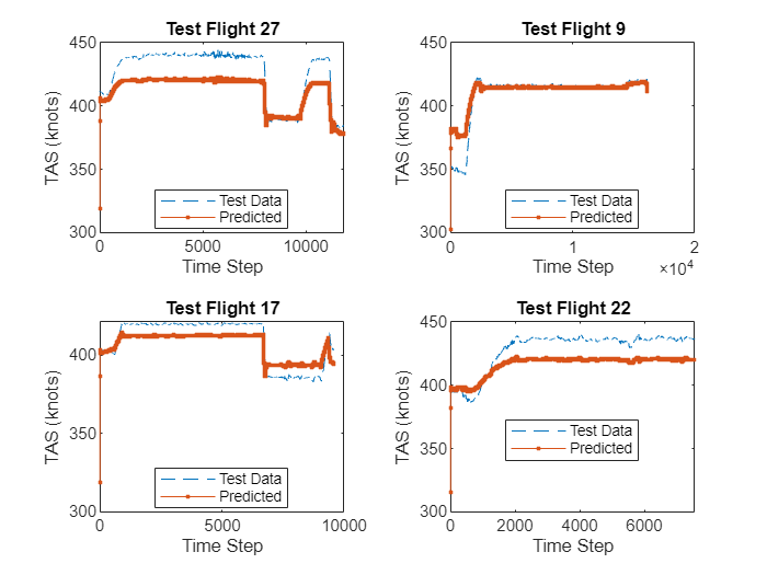
You can use the trained neural network to predict the true airspeed of each flight sequence in the test datastore. After the prediction is complete, convert the normalized predicted values to the real values.
yPred = minibatchpredict(net,tpdsTestPredictors,MiniBatchSize=1,UniformOutput=false);
minTAS = stats.min(5);
maxTAS = stats.max(5);
predictedTrueAirspeeds  = cellfun(@(x) (maxTAS-minTAS)*(x+minTAS),yPred,UniformOutput=false);
Extract the target true airspeed values for comparison. Set UseParallel to true to use the workers of the open parallel pool.
targetY = readall(tpdsTestTargets,UseParallel=true);
targetTrueAirspeeds = targetY.("Test Targets");
Compare the target and predicted true airspeed in a plot.
idx = randperm(length(predictedTrueAirspeeds),4);
figure
tiledlayout(2,2)
for i = 1:numel(idx)
    nexttile
    plot(targetTrueAirspeeds{idx(i)},"--")
    hold on
    plot(predictedTrueAirspeeds{idx(i)},".-")
    hold off
    title("Test Flight " + idx(i))
    xlabel("Time Step")
    ylabel("TAS (knots)")
    legend(["Test Data","Predicted"],Location="best")
end
Calculate the mean of the maximum absolute error, the maximum relative error (as a fraction of the target value) and the mean RMSE between the target and predicted true airspeed values.
absErrors = cellfun(@(x1,x2) max(abs(x1-x2)),targetTrueAirspeeds,predictedTrueAirspeeds);
maxRelativeError = cellfun(@(x1,x2) max((abs(x1-x2)./x1)),targetTrueAirspeeds,predictedTrueAirspeeds);
rootMeanSE = cellfun(@(x1,x2) rmse(x1,x2),targetTrueAirspeeds,predictedTrueAirspeeds);
meanAbsErrors = mean(absErrors);
fprintf("Mean maximum absolute error = %5.4f knots",meanAbsErrors)
Mean maximum absolute error = 79.2402 knots
meanRMSE = mean(rootMeanSE);
fprintf("Mean RMSE = %5.4f knots",meanRMSE)
Mean RMSE = 11.3948 knots
Plot the maximum absolute error for the test flight data.
figure
nexttile
histogram(rootMeanSE)
xlabel("RMSE (knots)")
ylabel("Frequency")
title("RMSE")
nexttile
histogram(maxRelativeError*100)
xlabel("Absolute Error (%)")
ylabel("Frequency")
title("Max Absolute Errors as Percentage of Target")

Clean Up
Remove the flight data files and delete the parallel pool.
rmdir(dataRoot,"s");
delete(pool);
References
[1] “Flight Data For Tail 652 | NASA Open Data Portal.” Accessed October 6, 2023. https://data.nasa.gov/dataset/Flight-Data-For-Tail-652/fxpu-g6k3.
See Also
parfor | fileDatastore | transform | writeall
Related Topics
You can also select a web site from the following list:
Americas
- América Latina (Español)
- Canada (English)
- United States (English)
Europe
- Belgium (English)
- Denmark (English)
- Deutschland (Deutsch)
- España (Español)
- Finland (English)
- France (Français)
- Ireland (English)
- Italia (Italiano)
- Luxembourg (English)
- Netherlands (English)
- Norway (English)
- Österreich (Deutsch)
- Portugal (English)
- Sweden (English)
- Switzerland
- United Kingdom (English)