Graph Signal Processing and Brain Signal Analysis

Graph signal processing (GSP) extends signal processing to analyze signals on nonuniform domains through weighted graphs, which are adept at representing complex and variable interactions between similar elements within a network. Graph signal processing is particularly useful for data sets where elements are interconnected by physical or functional relationships with varying degrees of intensity, such as brain regions, social networks, or weather stations. While some graphs depict clear, observable connections in various networks, other graphs capture implicit relationships that must be inferred from the data, reflecting dependencies or similarities.

This example shows how you can apply graph signal processing to perform a first-principles analysis of brain activity by constructing a graph from its structural connectivity and considering brain activity as graph signals. The example also shows how to do fundamental signal processing analysis on a brain graph, decompose the brain signals into aligned and liberal components, and identify which brain regions predominantly support these aligned and liberal activities. The aligned and liberal signals are analogous to low and high frequencies in classical Fourier analysis.

Download Data Set

This example uses the resting-state functional MRI (fMRI) data of one subject from the Human Connectome Project (HCP) Young Adult data set [1]. Perform these steps to download the preprocessed data of one subject:

1. Create an account on the ConnectomeDB platform.

2. Log in to the ConnectomeDB platform.

3. Install the IBM Aspera Connect plugin in your browser.

4. Accept the Open Access Terms for the WU-Minn HCP Data - 1200 Subjects.

5. For the WU-Minn HCP Data - 1200 Subjects data set, under Download Image Data, select the Single Subject option.

6. Download the Resting State fMRI FIX-Denoised data to the current working directory.

The data set is a ZIP file named 100206_3T_rfMRI_REST_fix.zip, and has a size of approximately 4 GB. Unzip the data set.

subjectNum = "100206";
unzip(subjectNum+"_3T_rfMRI_REST_fix.zip");

For each subject in the HCP S1200 dataset, resting-state fMRI data were collected in two sessions, each comprising two runs lasting about 15 minutes, where subjects kept their eyes open, focusing on a bright cross-hair against a dark backdrop in a dim room. Each session alternated between phase encoding directions: right-to-left (RL) in one run and left-to-right (LR) in the other. This example uses the fMRI file rfMRI_REST1_LR_Atlas_MSMAll_hp2000_clean.dtseries.nii which is captured in the first session with LR encoding and located in the directory 100206/MNINonLinear/Results/rfMRI_REST1_LR.

Extracting time series data from an fMRI file in the Human Connectome Project (HCP) requires a brain atlas. This example uses the HCP recommended atlas [2]. Perform these steps to download the atlas file:

1. Create an account on the Brain Analysis Library of Spatial maps and Atlases (BALSA) platform.

2. Login to the BALSA platform.

3. Navigate to the atlas page.

4. In the tab Data Use Terms, accept the WU-Minn HCP Consortium Open Access Data Use Terms.

5. Click on the tab Download File to download the atlas file named Q1-Q6_RelatedValidation210.CorticalAreas_dil_Final_Final_Areas_Group_Colors_with_Atlas_ROIs2.32k_fs_LR.dlabel.nii to the current working directory.

This example provides a helper function to read the fMR file and the atlas file and a function for extracting the brain signal.

Brain Network and Brain Signal

Brain networks describe physical connection patterns between brain regions. These connections are mathematically described by a weighted graph $$G=(V,A)$$ where $$V=\{0,1,\dots ,n-1\}$$is a set of $$n$$ nodes associated with specific brain regions and $$A\in {\mathbb{R}}^{n\times n}$$ is a weighted adjacency matrix with entries $$a_{ij}\ge 0$$ representing the strength of the physical connection between brain regions $$i$$ and $$j$$.

The brain regions encoded in the nodes $$V$$ are macroscale parcels of the brain that our current understanding of neuroscience deems anatomically or functionally differentiated. A brain parcel, also known as a region, is composed of adjacent brain areas that are spatially contiguous and similar in terms of topographical layouts, connectivity patterns, or functional networks. Segmenting the brain into these parcels is known as brain parcellation. The literature features a variety of brain parcellation maps, each with different resolutions and specific locations. A commonly used and publicly available parcellation is the HCP's multimodal parcellation (MMP) [2]. The HCP-MMP offers 180 cortical parcels for each hemisphere, resulting in a total of 360 regions (nodes) in the brain network. These nodes are categorized into 10 main functional networks [3],[4]. This table lists the names of the parcels, the functional networks, and the center coordinates of selected regions.

load("data/example_gsp_brain_signal_analysis.mat","brainRegions")
regionIdx = reshape([1 24]'+[0 180],[],1);
brainRegions(regionIdx,:)

ans=4×4 table
    Left or Right           Region Name           Network              Coordinates         
    _____________    _________________________    ________    _____________________________

                                                                 x          y          z   
                                                              _______    _______    _______
                                                                                           
          L          Primary_Visual_Cortex_L      Visual      -9.4505    -85.016    0.58242
          L          Primary_Auditory_Cortex_L    Auditory    -45.534    -24.447     10.505
          R          Primary_Visual_Cortex_R      Visual       11.139    -81.563     3.1055
          R          Primary_Auditory_Cortex_R    Auditory     45.237    -21.789     10.974

The element $$a_{ij}$$ of the adjacency matrix $$A$$ measures the strength of the axonal connection between region $$i$$ and region $$j$$. This strength is a simple count of the number of streamlines (estimated individual fibers) that connect the regions, and can be estimated with diffusion tensor imaging (DTI). This example uses a simple geometric-based model to generate the adjacency matrix of the brain network instead of applying tractography on the DTI data. This model relies on the fact that brain structural connectivity has to depend on distance due to the presence of physical constraints in the brain topology. In the geometric-based connectivity model, the strength of the connection between two regions is proportional to the inverse of the square distance between the regions [5]. The hModelBrainConnectivity function implements the geometric-based model of brain structural connectivity.

Coordinates = brainRegions.Coordinates{:,:};
A = hModelBrainConnectivity(Coordinates);

The figure below shows the logarithm of the adjacency matrix. The indices for cortical regions in the left hemisphere range from 1 to 180, while the indices for cortical regions in the right hemisphere extend from 181 to 360. The $$(i,j)$$-th element in this figure shows how strong region $$i$$ is connected to region $$j$$. The elements with larger weights have brighter colors and denote stronger connections. The presence of strong connections in the second and fourth quadrants indicates that cortical connectivity is primarily governed by connections within the same hemisphere (ipsilateral connectivity). Nonetheless, notable regions in the first and third quadrants exhibit strong connections across the opposite hemispheres (contralateral connectivity).

plotBrainConnectivity(A)

In addition to structural connectivity, it is also possible to capture a brain signal, a collection of measurements $$x_i$$ that reflect neuronal activity in each cortical region. For instance, an fMRI reading records the value $$x_i$$ that quantifies the level of neuronal activity in brain region $$i$$. The collection of $$n$$ measurements is grouped in the vector signal $$x={\left[\begin{array}{cccc}{x}_0& x_1& \dots & x_{n-1}\end{array}\right]}^T\in {\mathbb{R}}^n$$. Brain signals for all the $$n=360$$ brain regions are collected over $$T$$ successive time samples, resulting in the matrix $$X\in {\mathbb{R}}^{n\times T}$$, whose $$t$$-th column codifies brain activity at the $$t$$th time instance.

The hExtractBrainSignal function utilizes the hCIFTIReadData helper function to read CIFTI fMRI and atlas files that you have already downloaded. For more information on CIFTI files, see hCIFTIReadData in the Helper Function Section. The fMRI data is structured as a $$V\times T$$ matrix where $$V$$ represents the number of voxels, with each voxel corresponding to a distinct cubic segment of the brain tissue. The atlas file provides a mapping that links each voxel to its specific brain region. Using this mapping, the hExtractBrainSignal function extracts the time series for each brain region by detrending and normalizing the time series data from the voxels that form that particular region. This figure shows an example of a brain signal matrix.

X = hExtractBrainSignal(subjectNum);
plotBrainSignal(X)

A fundamental feature of the signal $$x$$ is the existence of an underlying pattern of structural or functional connectivity that couples its values at different brain regions. Since the network is undirected and symmetric, the weights $$a_{ij}$$ and $$a_{ji}$$ are the same for all $$(i,j)$$ pairs. These weights represent a measure of proximity or similarity between nodes $$i$$ and $$j$$. In terms of the signal $$x$$, this means that when the weight $$a_{ij}$$ is large, the signal values $$x_i$$ and $$x_j$$ tend to be related. Conversely, when the weight $$a_{ij}$$ is small, the signal values $$x_i$$ and $$x_j$$ are related only indirectly through their separate connections to other nodes.

Graph Signal Processing

Graph signal processing expands the scope of signal processing to signals on irregular domains encapsulated by weighted graphs. Graphs offer flexibility in modeling irregular interactions. Signals indexed by a graph are ideal for representing data that is associated with a set where either/simultaneously:

1. The elements of the set are of a similar type, such as regions in the brain's cortex, individuals in a social network, or meteorological stations over a large area.

2. There is a relation, either physical or functional, of closeness, influence, or association among the elements in the set.

3. The intensity of such a relation varies between each pair of items.

The underlying graph can represent a tangible network, such as those found in infrastructure, social settings, informational contexts, or biological systems, where connections are explicitly observable. However, the graph is not explicit in numerous instances since it embodies a concept of interdependency or likeness among nodes that requires the connections to be deduced from the data.

This example uses the conventional definitions of the degree and Laplacian matrices [6]. The degree matrix $$D\in {\mathbb{R}}_{+}^{n\times n}$$ is a diagonal matrix with its $$i$$th diagonal element $$D_{ii}=\sum _{j=0}^{n-1}{a}_{ij}$$. The Laplacian matrix is defined as the difference $$L\triangleq D-A\in {\mathbb{R}}^{n\times n}$$. The components of the Laplacian matrix are explicitly given by $$L_{ij}=-a_{ij}$$ and $$L_{ii}=\sum _{j=0}^{n-1}{a}_{ij}$$. The Laplacian is a real-valued positive semidefinite matrix. There are also several variants of the graph Laplacian [7], such as the symmetric normalized graph Laplacian $$L_{sn}=D^{-1/2}L{D}^{-1/2}$$ that factors out differences in degree and is thus only reflecting relative connectivity, or the random-walk normalized graph Laplacian $$L_{rw}=D^{-1}L$$. The eigenvector decomposition of $$L$$ is utilized in the following section to define the graph Fourier transform and the associated notion of graph frequencies.

Given the brain connectivity summarized in the adjacency matrix $$A$$, and the center coordinates of the brain regions, this example provides the MATLAB object signalSimpleGraph to construct the brain graph. Based on the specified adjacency matrix, the object specifies if the graph is weighted or not and if it is directed or not. signalSimpleGraph also computes the degree matrix and the Laplacian matrix based on the specified Laplacian type. This object can be used to create objects for an arbitrary graph.

brainGraph = signalSimpleGraph(A, ...
    Coordinates=Coordinates, ...
    LaplacianType="normalized-symmetric", ...
    Name="Brain Graph");

Using the specified coordinates and the function plotGraph in the object, the brain graph is shown in this figure where each point shows the center coordinate of a region.

plotGraph(brainGraph);

The function computeDegreeMatrix in the object signalSimpleGraph computes the degree of each node based on the provided adjacency matrix. The distribution of the weighted degrees of the nodes of the brain graph is illustrated below. The histogram shows that each region in the brain is approximately connected to 15 regions and that there are no zeroth-degee nodes that correspond to isolated regions.

plotBrainGraphDegreeDistribution(brainGraph.DegreeMatrix)

Use the function plotGraphSignal to plot the brain signal associated with the brain graph at 10 time instances. The amount of brain activity quantified by the signal amplitude is changing over this particular time interval.

fig = figure;
tl = tiledlayout(2,5);
for t = 500:509
    ax = nexttile(tl);
    plotGraphSignal(brainGraph,X(:,t), ...
        Figure=fig,Axes=ax,ShowColorbar=false);
    title(ax,sprintf("t = %d",t))
    axis(ax,"square")
end
title(tl,"Brain Signals")

Graph Fourier Transform, Graph Frequencies, and Graph Filtering

Given that the graph Laplacian $$L$$ is a real-valued symmetric matrix, it can be decomposed into its eigenvalue components

$$L=U\Lambda U^H$$

with eigenvalues $$\{{\lambda }_k\},k=0,1,\dots ,n-1$$. The diagonal eigenvalue matrix is defined as $$\Lambda =diag({\lambda }_0,{\lambda }_1,\dots ,{\lambda }_{n-1})$$, and $$U=\left[\begin{array}{cccc}{u}_0& u_1& \cdots & u_{n-1}\end{array}\right]$$is the eigenvector matrix. The eigenvector matrix $$U$$ is used to define the Graph Fourier Transform (GFT) of the graph signal $$x$$ [8]. Given a signal $$x\in {\mathbb{R}}^n$$ and a graph Laplacian $$L\in {\mathbb{R}}^{n\times n}$$, the GFT of $$x$$ with respect to $$L$$ is

$$\underset{}{\overset{\sim }{x}}=U^{H}x$$.

The inverse GFT (IGFT) of $$\underset{}{\overset{\sim }{x}}$$ with respect to $$L$$ is defined as $$x=U\underset{}{\overset{\sim }{x}}$$.

GFT encodes a notion of variability similar to the notion of variability that the Fourier transform encodes for temporal signals [9]. The eigenvectors of the graph Laplacian matrix provide a similar notion of frequency. Define the total variation of the graph signal $$x$$ with respect to the Laplacian $$L$$ as

$${\text{TV}}_G(x)=x^{H}Lx=\sum _{i\ne j}{a}_{ij}(x_i-x_j{)}^2$$.

The total variation $${\text{TV}}_G(x)$$ is a measure of how much the signal changes with respect to the network. For the edge $$(i,j)$$, when $$a_{ij}$$ is large it is expected that the values $$x_i$$ and $$x_j$$ to be similar because a large weight $$a_{ij}$$ encodes functional similarity between brain regions $$i$$ and $$j$$. The contribution of their difference $$(x_i-x_j{)}^2$$ to the total variation is amplified by the weight $$a_{ij}$$. If the weight $$a_{ij}$$ is small, activities at brain regions $$i$$ and $$j$$ tend to be uncorrelated, and therefore the difference between the signal values $$x_i$$ and $$x_j$$ makes little contribution to the total variation. Therefore, a signal with low total variation is seen as changing slowly on the graph, while one with high total variation changes rapidly.

The total variation of the eigenvectors $$u_k$$ is

$${\text{TV}}_G(u_k)=u_k^{H}L{u}_k={\lambda }_k$$

for $$k=0,\dots ,n-1$$. Since the eigenvalues are sorted as $$0={\lambda }_0\le {\lambda }_1\le \dots \le {\lambda }_{n-1}$$, the total variations of the eigenvectors $$u_k$$ follow the same order. When $$k$$ is close to 0, the eigenvectors $$u_k$$ vary slowly over the graph, whereas for $$k$$ close to $$n$$ the eigenvectors vary more rapidly. Section GFT and Classical Signal Processing in the Appendix illustrates the relationship between GFT and classical Fourier transform by modeling a time-series signal as a cycle graph and also discusses graph frequency and variability of eigenvectors across the graph.

When creating the object brainGraph, the object signalSimpleGraph computes the Laplacian matrix using the function computeLaplacianMatrix based on the specified LaplacianType. The object also computes the Fourier basis and eigenvalues of the Laplacian matrix of the brain graph using the function computeGraphFourierBasis. The figure below shows the eigenvalues (brain graph frequencies). As mentioned above, an eigenvalue quantifies how much variability the corresponding eigenvector has across the graph nodes. The larger the eigenvalue, the higher the variability of the corresponding eigenvector across the graph.

plotBrainGraphEigenvalues(brainGraph.NumNodes,brainGraph.Eigenvalues)

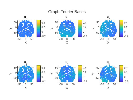
The figure shows the first 6 eigenvectors of the Laplacian matrix of the brain graph. The variability of eigenvectors across the brain increases as eigenvalues increase.

fig = figure;
tl = tiledlayout(2,3);
cLim = [min(brainGraph.FourierBases(:,1:6),[],"all")
        max((brainGraph.FourierBases(:,1:6)),[],"all")];
for i = 1:6
    ax = nexttile(tl);
    plotGraphSignal(brainGraph,brainGraph.FourierBases(:,i), ...
        Figure=fig,Axes=ax,ShowColorbar=true,ColorLim=cLim);
    title(ax,sprintf("u_{%d}",i-1))
    axis(ax,"square")
end
title(tl,"Graph Fourier Bases")

Given the GFT-IGFT relationship, it becomes possible to manipulate the graph signals by extracting signal components associated to different graph frequency ranges. Let $$\underset{}{\overset{\sim }{H}}$$ be the diagonal filtering matrix, where $${\underset{}{\overset{\sim }{H}}}_{kk}=\underset{}{\overset{\sim }{h}}({\lambda }_k)$$ is the frequency response for the graph frequency associated with eigenvalue $${\lambda }_k$$, and retrieve the filtered signals as $$\underset{}{\overset{\sim }{x}}=U\underset{}{\overset{\sim }{H}}{U}^{H}x$$. For the graph setting, define generic filtering operations such as ideal lowpass filtering, where $$\underset{}{\overset{\sim }{h}}({\lambda }_k)=1$$for $$k<K_L$$ and $$0$$ for all other indices beyond a certain cutoff index $$K_L,0\le K_L\le n-1$$. Similarly, define a generic graph highpass filter as $$\underset{}{\overset{\sim }{h}}({\lambda }_k)=1$$for $$K_H\le k$$ and $$0$$ for all other indices.

Using GFT and IGFT, the brain signal $$x$$ can be decomposed into components that characterize different levels of variability [10]. The GFT coefficients $${\underset{}{\overset{\sim }{x}}}_k$$ for small values of $$k$$ indicate how much these slowly varying signals contribute to the observed brain signal $$x$$ [11]. On the other hand, the GFT coefficients $${\underset{}{\overset{\sim }{x}}}_k$$ for large values of $$k$$ describe how much rapidly varying signals contribute to the observed brain signal $$x$$. So let's compute the GFT of the brain signal at hand.

Xt = brainGraph.gft(X);

Set the cutoff index to 20 and decompose the GFT of the brain signal in an aligned component, which corresponds to low frequencies, and a liberal component, which corresponds to high frequencies.

K = 20; % Cutoff index

Xta = Xt; % Align
Xta(K:end,:) = 0;
Xtl = Xt; % Liberal
Xtl(1:K-1,:) = 0;

Calculate and plot the align and liberal signals using IGFT.

Xa = brainGraph.igft(Xta);
Xl = brainGraph.igft(Xtl);
plotAlignedAndLiberalSignals(X,Xa,Xl)

Use the energy of the aligned and liberal signals as a feature to illustrate the distribution of alignment components and liberality components across the brain network. Compute the energy for each of these signals. Plot the computed energy for each signal on the brain graph.

Exa = sum(abs(Xa).^2,2);
Exl = sum(abs(Xl).^2,2);
plotEnergyAlignedAndLiberalSignals(brainGraph,Exa,Exl)

Since the Graph Fourier Transform (GFT) is applied to the brain signal at each time sample, this approach determines the location and degree to which brain signals throughout the brain conform to the structure of brain network. In the same way that a single brain region can exhibit a time series containing components at both low and high frequencies, a single brain region can also show elements that are both in sync (aligned) with and independent (liberal) from these networks.

As hypothesized in [12], the sensory regions, like visual and auditory, should correspond to the aligned activity, which means that functional signals are aligned with anatomical brain structure. On the other hand, regions involved in high-level cognition, like decision making and memory, correspond to liberal activity. The median energy for each brain functional group is used as a metric for sorting the amount of alignment and liberality. The function plotAlignedAndLiberalRegions groups the brain parcels that belong to the same functional network, e.g., visual, and sort these 10 functional groups based on the median energy.

plotAlignedAndLiberalRegions(Exa,Exl,brainRegions.Network)

Conclusion

The graph signal processing framework helps analyzing signals defined by graphs that represent similarity or dependency relations. In this example, the brain's structural connectivity serves as the graph for signals captured by functional MRI. Through the use of the Graph Fourier Transform (GFT) and its inverse (IGFT), the brain signal is separated into aligned and liberal components. This decomposition helps identify which brain regions predominantly support these aligned and liberal activities.

Appendix

GFT and Classical Signal Processing

In classical signal processing, a signal is sampled at regular, equally spaced intervals. The sequence of signal samples is straightforward, with each sample $$x(n)$$ being directly preceded by $$x(n-1)$$ and followed by $$x(n+1)$$. The time distance between samples is considered as the basic parameter in various processing algorithms. This relation between sampling instants can be represented in a graph form. The nodes correspond to the instants when the signal is sampled and the edges define node ordering. The fact that sampling instants are equally spaced can be represented with same weights for all edges (for example normalized to 1). Most digital signal processing algorithms assume periodicity of the analyzed signals, which means that $$x(0)$$ comes after $$x(N-1)$$. This case corresponds to a directed cycle graph. The figure shows the cycle graph model of a time signal with 8 samples. For the cycle graphs, the Laplacian matrix is a circulant matrix. Hence the eigenvectors are the columns of the DFT matrix. Further, the eigenvalues are a monotonically increasing function of the Fourier frequency and hence the GFT corresponds to the DFT conforming to our intuition.

Create a graph that models a periodic digital signal with 8 samples. The coordinates of the graph nodes are on a unit circle.

Nx = 8;
pointOnCircle = exp(1i*2*pi*mod((1:Nx)',Nx)/Nx);
dsCoordinates = [imag(pointOnCircle),real(pointOnCircle)];

The adjacency matrix of the graph can be generated using the function toeplitz. Note that the element $$a_{ij}$$ in the adjacency matrix of a directed graph is nonzero if there is an edge from node $$j$$ to node $$i$$.

dsA = toeplitz([0;1;zeros(Nx-2,1)],[zeros(1,Nx-1,1),1]);

Create the cycle graph for an 8-sample signal using the object signalSimpleGraph.

digitalSignalGraph = signalSimpleGraph(dsA, ...
    Coordinates=dsCoordinates, ...
    LaplacianType="combinatorial");

Visualize the graph using the function plotGraph.

fig = figure;
ax = axes(Paren=fig);
digitalSignalGraph.plotGraph( ...
    NodeSize=100,ShowEdge=true, ...
    Figure=fig,Axes=ax);
text(ax, ...
    0.95*dsCoordinates(:,1)-0.05, ...
    0.95*dsCoordinates(:,2), ...
    arrayfun(@(l) {sprintf('x(%d)',l)},0:Nx-1))
axis(ax,"square")

Plot the eigenvectors of the graph. Move the slider and observe how eigenvectors vary across the graph. As you increase the index of the Fourier basis, the frequency of the eigenvector increases and, in turn, variability of the corresponding eigenvector across the graph, shown at the bottom plot, increases. When idx is set to 1, the corresponding eigenvalue is $${\lambda }_0=0$$, so the corresponding eigenvector $$u_0$$ is just a constant and it has no variability across the graph. However, if idx is set to 8, which corresponds to the largest eigenvalue $${\lambda }_7$$, then the corresponding eigenvector $$u_7$$ exhibits the maximum variability across the graph and thus has highest frequency.

idx = 1;
plotDigitalSignalGraphFourierBases(digitalSignalGraph,idx)

Helper Functions

The functions listed in this section are only for use in this example. They may change or be removed in a future release.

hModelBrainConnectivty

This function models the structural connectivity of the brain based on the distance between center coordinates of brain regions.

function A = hModelBrainConnectivity(Coordinates)
% Compute pairwise distance
C = Coordinates';
pd = computePairwiseDistance(C);
% Compute correlation based on power law
d0 = mean(pd);
gamma = 2;
W0 = 1;
corr = 1./(W0.*(pd./d0).^gamma);

% Create structural connectivity
A = convertToSquareMatrix(corr);
end

function d = computePairwiseDistance(C)
% Compute pairwise Euclidean distance
D = dot(C,C,1)+(dot(C,C,1)')-2*(C'*C);
% To make sure there is no negative element due to numerical rounding, the
% negative elements are set to 0
D(D < 0) = 0;
D = sqrt(D);
% Create a lower triangular matrix with all the elements below the main
% diagonal
Dlt = tril(D,-1);
% Find index of lower triangular elements
ltIdx = (1:size(Dlt,1)) < (1:size(Dlt,2)).';
d = Dlt(ltIdx);
end

function S = convertToSquareMatrix(d)
N = numel(d); % N must be a triabular number, i.e. N = n*(n-1)/2
n = ceil(sqrt(2*N)); % (1+sqrt(1+8*N))/2
% Create a symmetric square matrix from vector d
S = zeros(n);
S(tril(true(n),-1)) = d;
S = S+S.';
end

hExtractBrainSignal

The hExtractBrainSignal function uses the helper function hCIFTIReadData to read the fMRI file and the atlas file that you already downloaded in the current working directory. The hExtractBrainSignal function extracts the time series of each brain region after detrending and normalizing time series of the voxels that construct the underlying brain region.

function X = hExtractBrainSignal(subjectFolder)

% Read atlas file
atlasFilename = "Q1-Q6_RelatedValidation210."+ ...
    "CorticalAreas_dil_Final_Final_Areas_Group_Colors_"+ ...
    "with_Atlas_ROIs2.32k_fs_LR.dlabel.nii";
atlasData = hCIFTIReadData(atlasFilename);

% In HCP MMP 1.0 atlas, the first 59412 elements correspond to the cortical
% region and the rest correspond to subcortical regions
corticalRegionIdx = 1:59412;
% In HCP MMP 1.0 atlas, there are 360 cortical regions
rois = unique(atlasData(corticalRegionIdx));
numRois = length(rois);

% Read fMRI file
fmriDataFolder = fullfile(subjectFolder,"MNINonLinear", ...
    "Results","rfMRI_REST1_LR");
fmriDataFile = "rfMRI_REST1_LR_Atlas_MSMAll_hp2000_clean.dtseries.nii";
fmriData = hCIFTIReadData(fullfile(fmriDataFolder,fmriDataFile));
% The data is N-by-T where N is the number of voxels
numTimeSamples = size(fmriData,2);

X = zeros(numRois,numTimeSamples);
for nr = 1:numRois
    % Find the indexes in the atlas that correspond to one of the 360 ROIs
    % in the HCP MMP 1.0 atlas
    ridx = (atlasData == rois(nr));

    % Extract the corresponding time series
    regionsSig = fmriData(ridx,:);

    % Normalize and detrend the signals
    m = mean(regionsSig,2);
    s = std(regionsSig,[],2);
    normalizedRegionSig = (regionsSig-m)./s;
    detrendRegionSig = detrend(normalizedRegionSig',1);

    % Take the average and normalize the ROI signal
    roiSig = mean(detrendRegionSig,2);
    roiSig = (roiSig-mean(roiSig))/std(roiSig);
    X(nr,:) = roiSig;
end
% Remove the first 10 time samples so the magnetic resonance signal reaches
% steady state
X = X(:,11:end);
end

hCIFTIReadData

The hCIFTIReadData function reads matrix of values stored in a Connectivity Informatics Technology Initiative (CIFTI-2) file [13]. A CIFTI-2 file has a header which is represented in a NIFTI-2 format [14]. The downloaded fMRI and atlas files are in standardized CIFTI-2 formats. The helper function hCIFTIReadData extracts the important fields in the NIFTI-2 header which are required for extracting the matrix of the data from the file. The NIFTI-2 header is a binary block at the beginning of a CIFTI-2 file that contains essential metadata for interpreting the neuroimaging data, such as the data type, the data array dimensions, and the location in the file where the data matrix begins. This table shows how the NIFTI-2 format specifies these fields in the header structure.

Field	Data Type	Size	Offset from Beginning of File (BoF)	Description
datatype	int16	[1 1]	12	Data type of data matrix
dim	int64	[1 8]	16	Dimensions of data array
vox_offset	int64	[1 1]	168	File location where data matrix begins

function data = hCIFTIReadData(filename)
arguments
    filename {mustBeFile}
end

% Read NIFI-2 header
[fid,fcleanup,info] = extractCIFTIInfo(filename);

% Extract matrix of data
data = extractCIFTIData(fid,fcleanup,info);
end

function [fid,fcleanup,info] = extractCIFTIInfo(filename)

% In CIFTI files, order for reading is typically little-endian
[fid,errMsg] = fopen(filename,"rb","l");
% Make sure the file is opened
if fid < 0
    error(errMsg)
end
fcleanup = onCleanup(@()fclose(fid));

% Set the file position indicator for reading datatype
fid = setFilePositionIndicator(fid,12,"datatype");

% Read datatype and find stored datatype (source data type)
datatype = fileRead(fid,[1 1],"int16=>int16");
switch datatype
    case 16
        srctype = "float32";
    otherwise
        error("Not supported data type.");
end

% Set the file position indicator for reading dim
fid = setFilePositionIndicator(fid,16,"dim");

% Read dim and find data array dimensions
dim = fileRead(fid,[1 8],"int64=>int64");
if dim(1) < 1 || dim(1) > 7
    error("Header information needs to be byte swapped appropriately.");
end
if dim(1) < 6 || any(dim(2:5) ~= 1)
    error("Invalid dimensions.");
end
% dim(1) is 6 or 7, depending on whether a third matrix dimension
if (dim(1) ~= 6)
    error("CIFTI-2 files with 3D data are not supported.")
end

% Set the file position indicator for reading vox_offset
fid = setFilePositionIndicator(fid,168,"vox_offset");

% Read vox_offset (offset into matrix of data in .nii file)
voxOffset = fileRead(fid,[1 1],"int64=>int64");
if voxOffset < 544
    error("Offset into data must be greater than or equal to 544.");
end

% Read scaling parameters
scl_slope = fileRead(fid,[1 1],"double=>double");
scl_inter = fileRead(fid,[1 1],"double=>double");

% Set the file position indicator for reading matrix of values
fid = setFilePositionIndicator(fid,voxOffset,"data");

% Construct struct info
info = struct("dim",dim(:)', ...
              "srctype",srctype, ...
              "scl_slope",scl_slope, ...
              "scl_inter",scl_inter);
end

function data = extractCIFTIData(fid,fcleanup,info)

% Find out if scaling is needed
needScaling = ~(info.scl_slope == 0 || ...
    (info.scl_slope == 1 && info.scl_inter == 0));

% Read data in frames with maximum frame length of 64 MiB
maxFrameLen = 64*2^20;
if prod(info.dim(6:(info.dim(1)+1))) <= maxFrameLen
    % Small file
    data = fileRead(fid,info.dim(6:(info.dim(1)+1)), ...
        info.srctype+"=>float32");
    if needScaling
        data = (info.scl_slope).*data + (info.scl_inter);
    end
    data = permute(data,[2 1 3:(info.dim(1)-4)]);
else
    % Extract CIFTI dimensions from header:
    %   - data is an N-by-T matrix, where T is number of samples in 
    %     time and N is number of channels
    %   - Stored data matrix in CIFTI file is a T-by-N matrix
    dims = info.dim(6:(info.dim(1)+1));
    dims = dims([2 1 3:length(dims)]);
    if isscalar(dims)
        data = zeros(dims(1),1,"single");
    else
        data = zeros(dims,"single");
    end
    numColsPerRead = max(1,min(info.dim(7), ...
        floor(maxFrameLen/info.dim(6))));
    numRead = ceil(info.dim(7)/numColsPerRead);
    readHopLen = ceil(info.dim(7)/numRead);
    for n = 1:readHopLen:info.dim(7)
        dn = fileRead(fid, ...
            [info.dim(6),min(readHopLen,info.dim(7)-n+1)], ...
            info.srctype+"=>float32");
        if needScaling
            dn = (info.scl_slope).*dn+(info.scl_inter);
        end
        data(n:min(info.dim(7),n+readHopLen-1),:) = dn';
    end
end
fcleanup();
end

function vals = fileRead(fid,sizeA,precision)
[vals,numRead] = fread(fid,sizeA,precision);
if numRead ~= prod(sizeA)
    error("Fewer elements are read than expected.");
end
end

function fid = setFilePositionIndicator(fid,offset,fieldname)
if feof(fid)
    error("CIFTI-2 file is too short to contain "+ ...
        "the entire NIFTI-2 header.");
end
if (fseek(fid,offset,"bof") ~= 0)
    error("Failed to set file position indicator to "+ ...
        "the beginning of the field %s.",fieldname);
end
end

Plotting Helper Functions

function plotBrainConnectivity(A)
figure
imagesc(log(A));
colorbar;
cbar = colorbar;
cbar.Label.String = "log(A)";
title("Connectivity Weights of Brain Regions (log scale)")
xlabel("Brain Region Index (Left: 1-180 - Right: 181-360)")
ylabel("Brain Region Index (Left: 1-180 - Right: 181-360)")
end

function plotBrainSignal(bs)
figure
imagesc(bs)
colorbar
title("Brain Signal")
xlabel("Time (sample)")
ylabel("Brain Region Index")
end

function plotBrainGraphDegreeDistribution(D)
figure
histogram(diag(D),100)
xlabel("Node Degree")
ylabel("Count")
grid("on")
end

function plotDigitalSignalGraphFourierBases(digitalSignalGraph,idx)
U = digitalSignalGraph.FourierBases;
Lambda = digitalSignalGraph.Eigenvalues;

Nx = size(U,1);

fig = figure;
tl = tiledlayout("flow");
yLim = [-1.1 1.1]*max(abs(U(:)));
ax = nexttile(tl);
plot(ax,0:Nx-1,real(U(:,idx)),"-o")
title(ax,sprintf("u_{%d}, |\\lambda_{%d}| = %.4f", ...
    idx-1,idx-1,abs(Lambda(idx))))
xlabel(ax,"Node Index")
ylabel(ax,sprintf("\\Re \\{u_{%d}\\}",idx-1))
ylim(ax,yLim)
grid(ax,"on")

ax = nexttile(tl);
digitalSignalGraph.plotGraphSignal(real(U(:,idx)), ...
    Figure=fig,Axes=ax, ...
    NodeSize=600, ...
    ColorLim=yLim, ...
    ShowColorbar=true, ...
    ColorbarTitle=sprintf("\\Re \\{u_{%d}\\}",idx-1), ...
    ApplyAxisLim=false)
xlabel(ax,"X")
ylabel(ax,"Y")
text(ax,0.95*digitalSignalGraph.Coordinates(:,1)-0.05, ...
        0.95*digitalSignalGraph.Coordinates(:,2), ...
    arrayfun(@(l) {sprintf('%d',l)}, ...
    0:size(digitalSignalGraph.Coordinates,1)-1))
axis(ax,"square")
end

function plotBrainGraphEigenvalues(n,lambda)
figure
plot(1:n,lambda,"-o",LineWidth=2)
xlabel("Index k")
ylabel("Eigenvalue of Laplacian Matrix \lambda_{k}")
grid("on")
end

function plotAlignedAndLiberalSignals(X,Xa,Xl)
figure
tl = tiledlayout("vertical");

nexttile(tl)
imagesc(X)
colorbar
title("Brain Signal")

nexttile(tl)
imagesc(Xa)
colorbar
title("Aligned Signal")

nexttile(tl)
imagesc(Xl)
colorbar
title("Liberal Signal")

xlabel(tl,"Time (sample)")
ylabel(tl,"Brain Region Index")
end

function plotEnergyAlignedAndLiberalSignals(brainGraph,l2Xa,l2Xl)
fig = figure;
tiledlayout("horizontal");
ax = nexttile;
plotGraphSignal(brainGraph,l2Xa, ...
    NodeSize=500, ...
    Figure=fig, ...
    Axes=ax, ...
    ShowColorbar=true)
title(ax,"Energy of Aligned Signal")
axis(ax,"square")

ax = nexttile;
plotGraphSignal(brainGraph,l2Xl, ...
    NodeSize=500, ...
    Figure=fig, ...
    Axes=ax, ...
    ShowColorbar=true)
title(ax,"Energy of Liberal Signal")
axis(ax,"square")
end

function plotAlignedAndLiberalRegions(Exa,Exl,Network)

% Alignment
Ta = table(Network,Exa,VariableNames=["Network" "Energy"]);
Ta = sortrows(Ta,"Energy");
Ta = convertvars(groupsummary(Ta,"Network","median","Energy"), ...
    "Network","categorical");
Ta = sortrows(Ta,"median_Energy","ascend");

% Liberality
Tl = table(Network,Exl,VariableNames=["Network" "Energy"]);
Tl = sortrows(Tl,"Energy");
Tl = convertvars(groupsummary(Tl,"Network","median","Energy"), ...
    "Network","categorical");
Tl = sortrows(Tl,"median_Energy","ascend");

figure
barh(string(Ta.Network),Ta.median_Energy)
xlabel("Alignment")
ylabel("Brain Functional Networks")

figure
barh(string(Tl.Network),Tl.median_Energy)
xlabel("Liberality")
ylabel("Brain Functional Networks")
end

Acknowledgment

Data were provided [in part] by the Human Connectome Project, WU-Minn Consortium (Principal Investigators: David Van Essen and Kamil Ugurbil; 1U54MH091657) funded by the 16 NIH Institutes and Centers that support the NIH Blueprint for Neuroscience Research; and by the McDonnell Center for Systems Neuroscience at Washington University.

References

[1] Van Essen, David C., Stephen M. Smith, Deanna M. Barch, Timothy E.J. Behrens, Essa Yacoub, and Kamil Ugurbil. “The WU-Minn Human Connectome Project: An Overview.” NeuroImage 80 (October 2013): 62–79. https://doi.org/10.1016/j.neuroimage.2013.05.041.

[2] Glasser, Matthew F., Timothy S. Coalson, Emma C. Robinson, Carl D. Hacker, John Harwell, Essa Yacoub, Kamil Ugurbil, et al. “A Multi-Modal Parcellation of Human Cerebral Cortex.” Nature 536, no. 7615 (August 2016): 171–78. https://doi.org/10.1038/nature18933.

[3] Rosen, Burke Q., and Eric Halgren. “A Whole-Cortex Probabilistic Diffusion Tractography Connectome.” Eneuro 8, no. 1 (January 2021): ENEURO.0416-20.2020. https://doi.org/10.1523/ENEURO.0416-20.2020.

[4] Patterson, Dianne. “Atlases.” Atlases. readthedocs.io, July 16, 2023. https://neuroimaging-core-docs.readthedocs.io/en/latest/pages/atlases.html

[5] Perinelli, Alessio, Davide Tabarelli, Carlo Miniussi, and Leonardo Ricci. “Dependence of Connectivity on Geometric Distance in Brain Networks.” Scientific Reports 9, no. 1 (September 16, 2019): 13412. https://doi.org/10.1038/s41598-019-50106-2.

[6] Chung, Fan R. K. Spectral Graph Theory. Regional Conference Series in Mathematics, no. 92. Providence, R.I: Published for the Conference Board of the mathematical sciences by the American Mathematical Society, 1997.

[7] Ortega, Antonio. Introduction to Graph Signal Processing. New York, NY: Cambridge University Press, 2021.

[8] Shuman, D. I., S. K. Narang, P. Frossard, A. Ortega, and P. Vandergheynst. “The Emerging Field of Signal Processing on Graphs: Extending High-Dimensional Data Analysis to Networks and Other Irregular Domains.” IEEE Signal Processing Magazine 30, no. 3 (May 2013): 83–98. https://doi.org/10.1109/MSP.2012.2235192.

[9] Segarra, Santiago, Antonio G. Marques, Geert Leus, and Alejandro Ribeiro. “Reconstruction of Graph Signals Through Percolation from Seeding Nodes.” IEEE Transactions on Signal Processing 64, no. 16 (August 15, 2016): 4363–78. https://doi.org/10.1109/TSP.2016.2552510.

[10] Huang, Weiyu, Thomas A. W. Bolton, John D. Medaglia, Danielle S. Bassett, Alejandro Ribeiro, and Dimitri Van De Ville. “A Graph Signal Processing Perspective on Functional Brain Imaging.” Proceedings of the IEEE 106, no. 5 (May 2018): 868–85. https://doi.org/10.1109/JPROC.2018.2798928.

[11] Huang, Weiyu, Leah Goldsberry, Nicholas F. Wymbs, Scott T. Grafton, Danielle S. Bassett, and Alejandro Ribeiro. “Graph Frequency Analysis of Brain Signals.” IEEE Journal of Selected Topics in Signal Processing 10, no. 7 (October 2016): 1189–1203. https://doi.org/10.1109/JSTSP.2016.2600859.

[12] Medaglia, John D., Weiyu Huang, Elisabeth A. Karuza, Apoorva Kelkar, Sharon L. Thompson-Schill, Alejandro Ribeiro, and Danielle S. Bassett. “Functional Alignment with Anatomical Networks Is Associated with Cognitive Flexibility.” Nature Human Behaviour 2, no. 2 (December 18, 2017): 156–64. https://doi.org/10.1038/s41562-017-0260-9.

[13] NeuroImaging Tools and Resources Collaboratory . “CIFTI Connectivity File Format,” December 18, 2013. https://www.nitrc.org/projects/cifti.

[14] Neuroimaging Informatics Technology Initiative. “NIfTI-2 Data Format,” December 18, 2013. https://nifti.nimh.nih.gov/nifti-2.